

YouTube's RecSys paper is a box of insights
Every ML Engineer can learn from YouTube's recommendation algorithm

In this article, we dive into YouTube’s recommender system as described in their paper Deep Neural Networks for YouTube Recommendations.
Before I get into the paper, let me set some context. YouTube’s recommender system works in two stages - 1. Candidate Generation 2. Ranking. The candidate generation stage uses lightweight models to score millions of videos (from the database) for a user. The top thousands form a probable set of relevant videos. The ranking stage then uses a heavier model with more features to score these thousands of videos and sorts them according to their score. The top few videos form the final set of recommendations shown to the user.

Instead of going deep-diving into the paper linearly, I elaborate on essential design decisions the authors took in a widely applicable way to most ML problems.
Posing recommendations as a classification problem
Training data for any recommendation model occurs as a list of (userId, itemId) pairs, indicating the occurrence of an action (click, watch, purchase) performed by the user on an item. During training, the score is computed for each pair and then the subsequent loss.

From a lens of binary classification, the model only sees the positive classes, i.e., occurrence of an event. There is no clear definition of a negative class, as we can only record events that occurred. However, YouTube decided to treat this problem as a multiclass classification. If I just mentioned that we observe only the positive class, how can we formulate recommendations as a binary classification, let alone multiclass? The solution is sampling negative examples from the distribution of videoIds in the training data distribution.

For a (userId, videoId) pair, sample, say 1000 randomly selected videoIds , which form negative examples for the concerned pair. Instead of producing scores for 1001 pairs separately, compute softmax over these 1001 ‘classes.’
Each score can be between 0 and 1 in the former scoring pattern. However, all the 1001 scores must sum to 1 in the latter.
Consolidating variable-length user history
The model uses features derived from a user’s watch history as inputs. The number of past watches differs for every user. If user A has 20 videos in their history and user B has 30, the input features are of sizes 20x256 and 30x256, assuming a 256-dimensional embedding represents each video.
Since inputs to a feed-forward neural network are fixed size, the paper recommends taking an average over the history, or component-wise max, to summarize the history information into single, fixed-sized embedding.
Adding temporal flair to the model
Among many features used to score a video for a user, the age of the training example is one of them. This feature is calculated as the time difference between a video-watch event and the end of the training window.
If the training window ends at ‘13-06-2023 13:00:00’, a video watch occurring at ‘13-06-2023 12:37:00’ has 23 minutes as the example-age. The interesting question is, what happens during inference? In inference, the ‘end of the window’ is literally the timestamp of the event in question. Hence, the value of the feature is 0. Semantically, it tells the model to leverage the knowledge it acquired when training on the latest examples (with an example-age feature close to zero).
The effect they observed in the model’s learning patterns is intriguing. Each newly uploaded video garners some popularity in the initial few days, after which it drops. It’s difficult for traditional collaborative filtering to model such behavior since it uses no time-based feature. However, infusing the example age in the model did the trick. During training, a recently uploaded video must have a smaller average (over all its watches) example-age, and most watches are concentrated around this spike.
Conversely, an older video must have a larger average example-age, with watches more spread out. In inference, since we use 0 as the example age, the model must infer from the distribution of this spike. The inference is business-as-usual since there is no spike for the older video.

Training data precautions
A model that only trains on the feedback from its recommendations degrades very quickly. At first, it recommends items that most certainly have a popularity bias and then learns from feedback on these biased items, which leads to the compounding of this bias. Hence, it needs feedback from other sources that don’t depend on it. Otherwise, learning relevance for new items or even niche, long-tailed items becomes difficult. In this case, YouTube uses feedback logs from other sources, like websites that embed YouTube videos. This allows the model training to infuse information from diverse sources.
Fixing the number of training examples per user
Most marketplace platforms like YouTube follow a power law distribution. A small subset of users account for a significant portion of the activity. Training a collaborative filtering model on a skewed distribution may result in sub-optimal learning for the remaining users having scant activity. Hence, the authors decided to cap the number of training events they use per user.
Preventing the model from exploiting the platform structure
Consider a user entering the search query taylor swift songs. The user will likely click on many search results, most of which would be about Taylor Swift. A model trained to predict the next watch, given previous history, will receive this information in two ways—one, as a sequence of past watches, and the second, as search query embeddings. Consequently, the model learns to infer from this input-output pair that the next watch will likely be a Taylor Swift video and recommends it on the homepage. However, this isn’t optimal, as the user already got what they wanted. They don’t want to watch any more Taylor Swift videos, even though they did in the near past.
The authors suggest removing such videoIds from the input sequence and represent the search queries with an unordered bag of tokens. As a result, it becomes difficult for the model to pinpoint a piece of input and hack the next watch prediction probabilities. Now, the model learns that the user is a swiftie without exploiting the platform structure.
A better way to create a validation set
In a typical train-val split, the dataset is randomly split into training and validation sets. Such an approach works for IID (Independent and Identically Distributed) datasets. However, the assumptions in IID don’t hold in the recommendations dataset.
Hence, randomly sampling events to create a validation set is not optimal. If a user has 20 video watches, of which the 9th watch is included in the validation set, then the training loop has access to the 10-20th watch. The result is a data leak as the model can peep into the future to predict a past event.
A more sensible approach is to use a user’s last watch as a validation example. Remember that our model is trained to predict the next watch. In addition, certain asymmetric co-occurrences are better captured. If a user watches the first episode of a series, the next watch is most likely to be the second episode. Such a relationship is better captured in the described approach to the validation set.
Feature normalization is critical for convergence.
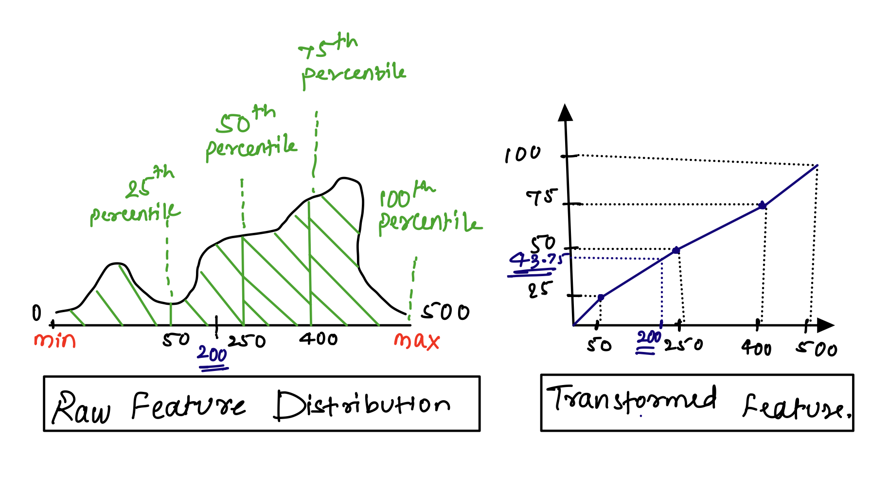
The authors used a quantile-based normalization, transforming a continuous feature into uniformly distributed values. The first step is to compute the quantiles of the raw features. Then, map each value in the feature to an approximate quantile value via interpolating on computed quantiles.
Modeling expected watch time instead of clicks
Instead of just modeling whether a user will click on a video, the authors model the time they will watch it. Using a weighted logistic regression, each positive example is weighted by the observed watch time. Conversely, this weight is set to one for negative examples.
Measuring the success of the expected watch time model
Authors measure per-user-loss to compare the performance of different model architectures. It measures how well the model captures expected watch time. For a positive example (shown to the user, and a click event occurred) and a negative example (shown to the user, but they did not click), if the negative example receives a greater score, the watch time on the positive example is treated as mispredicted watch time. In simpler terms, it measures how expensive this missed opportunity is.
However, it is not clear how these pairs are mined. Is it pairing random positives with random negatives? It sounds like ROC-AUC but with weights on the examples. In either case, the idea is interesting.
Closing thoughts
The best part about this paper is that it proposes improvements in the system by challenging assumptions and making corrections to it instead of focusing on fancy architectures.
YouTube engineers also released another fresh paper about their RecSys improvements a month back (link). Check it out if you are curious.
If the article helped you become slightly better at ML, consider supporting my substack.
If you think a friend or a colleague will find this article useful, share it with them.