Simplest explanation on hierarchical softmax
How hierarchical softmax speeds up inference in languge models. Why does it work, how does it work and everything in between.
The article is heavily inspired by the paper - A Scalable Hierarchical Distributed Language Model
Predicting the next word is expensive. Why?
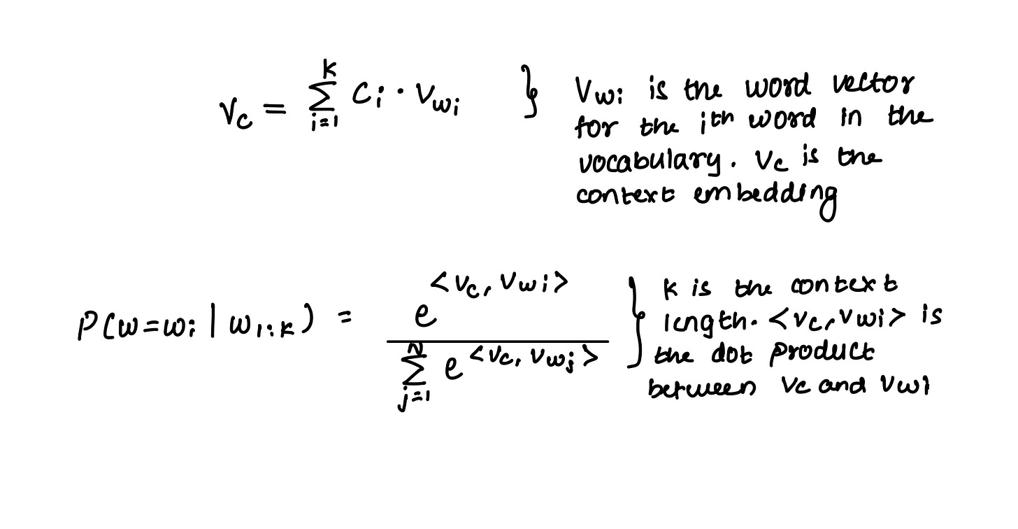
Almost every language model that trains to predict a word from the vocabulary is susceptible to a well-known computational bottleneck - predicting the word involves computing probabilities over the ENTIRE vocabulary. To look at it closely, consider a simple word embedding-based language model. The model takes a context of N consecutive words and performs a weighted sum of the corresponding N embeddings, producing a context embedding to predict the next word. It does so by computing the dot product with the word embeddings of the complete vocabulary and applying softmax on top. The word with the highest softmax score is chosen as the next word.

The softmax involves O(d*N) operations, where d is the embedding dimension. Vocabulary sizes are really large (in the order of 100,000s). Consequently, the above task is equivalent to performing a multi-class classification with thousands of classes. Vocabulary size limits how much we can scale the embedding dimension. To get an estimate, try executing the code below.
import numpy as np
import time

def compute_softmax_dot_products(matrix, vector):
    dot_products = np.dot(matrix, vector)
    exp_dot_products = np.exp(dot_products)
    softmax_values = exp_dot_products / np.sum(exp_dot_products)
    return softmax_values.argmax()

def main():
    # Define the size of vocabulary and dimensionality
    vocab_size = 100000  # Example: vocabulary size
    dimension = 100  # Example: dimensionality of vectors

    # Generate random matrix of size (vocab_size, dimension)
    matrix = np.random.randn(vocab_size, dimension)

    # Generate random vector of size dimension
    vector = np.random.randn(dimension)

    # Measure time taken for computation
    start_time = time.time()
    softmax_values = compute_softmax_dot_products(matrix, vector)
    end_time = time.time()
    time_taken = end_time - start_time

    print("Softmax over dot products computed successfully.")
    print("Time taken: {:.4f} seconds".format(time_taken))

    return time_taken
Computing softmax for a 100 dimension context embedding and a 100,000-sized vocabulary takes 0.018 seconds. This does not include the time taken to compute the context embedding itself.
Most vocabulary is useless in predicting the next word.
When computing the full softmax, the resulting probability distribution is usually skewed. This means that out of thousands of possible words, only a handful are plausible choices, which is logical. Most English words don’t fit in the blank - I love to play ____. Yet, we compute the probabilities for the entire vocabulary. This is suboptimal.
Can we avoid computing the probability of obviously unlikely words? The answer is yes, and this is what hierarchical softmax achieves.
What is hierarchical softmax?
Hierarchical softmax as a decision-making mechanism.
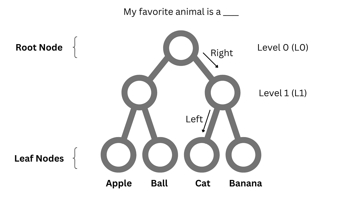
Imagine a balanced binary tree where all the leaf nodes are situated at the same level.
Every leaf node has a fixed path from the root node. This path is a series of steps, and each step entails a decision on whether to go right or left from the current node. In addition, the depth of the tree and the number of non-leaf nodes depend on the number of leaf nodes. Specifically, the depth of the tree is log2(N) + 1 where N is the number of leaf nodes. Note that this depth equals the number of decisions required to go from a root node to a leaf node.
Now, we adapt the tree to our problem. We assign each word in the vocabulary to a leaf node. Hence, the number of leaf nodes is equal to the vocabulary size. For example, if the vocabulary is [apple, ball, cat, banana] the tree looks like -
Given a context, can we begin at the root node and land on the next word? For example, in the figure below, the predicted word for the sentence My favorite animal is a ___ is cat, which is reached by taking a right and then a left from the root node.

Why would we want this? Computing a softmax over the entire vocabulary involves evaluating N words. Using a tree, we need log2(N) evaluations. To give you an estimate, for a vocabulary size of 100,000, this number is 17!
What are these evaluations and how does the navigation work?
So far, the model has two sets of parameters - word embeddings and the weights. We introduce another set of weights to this set. These weights are embeddings of the same dimension assigned to each non-leaf node (except the root node). The number of such embeddings in a tree is E = 2^0 + 2^1 + 2^2 + … + 2^(log2(N) - 1). So, the total number of additional parameters is E*d.
For a context embedding, we start at the root node and compute the probability of taking a right with its embeddings as
Conversely, the probability of taking a left is 1 minus this probability. If the probability is > 0.5, we take a right and move to the next node. Following this, we compute the probability of taking a right using the context embedding and the next node’s embeddings. The process is repeated till we reach a leaf node, which is our prediction. In total, we perform O(D) dot products, which is a lot less than performing O(N) dot products.
How is the tree trained?
When training the model, all three sets of parameters are trained jointly. A training pair comprising a context and the next word is trained by maximizing the log-likelihood. Given the context, probability is computed as the probability of taking the path from the root node to the next word’s leaf node. The probability of this path can be further broken down as the product of making individual decisions. In the above figure, this probability is
How is the tree constructed?
We introduced the binary tree without questioning its structure, how it was constructed, or how it affects its performance.
Let’s start with a thought experiment. What if the vocabulary was assigned to the leaf nodes randomly? Technically, such an assignment should work as each word has a unique path; thus it can be reached.
However, is it optimal?
Let’s step back and look at a similar problem in decision trees. The split in decision trees occurs based on the feature that results in the cleanest separation. In the case of binary classification, a split aims to separate the points of one class from the other, measured by information gain. In addition, the feature that results in most separation is picked first so that the chances of error are the least at the top of the tree, which makes sense as the quality of subsequent splits depends on that of previous splits'.
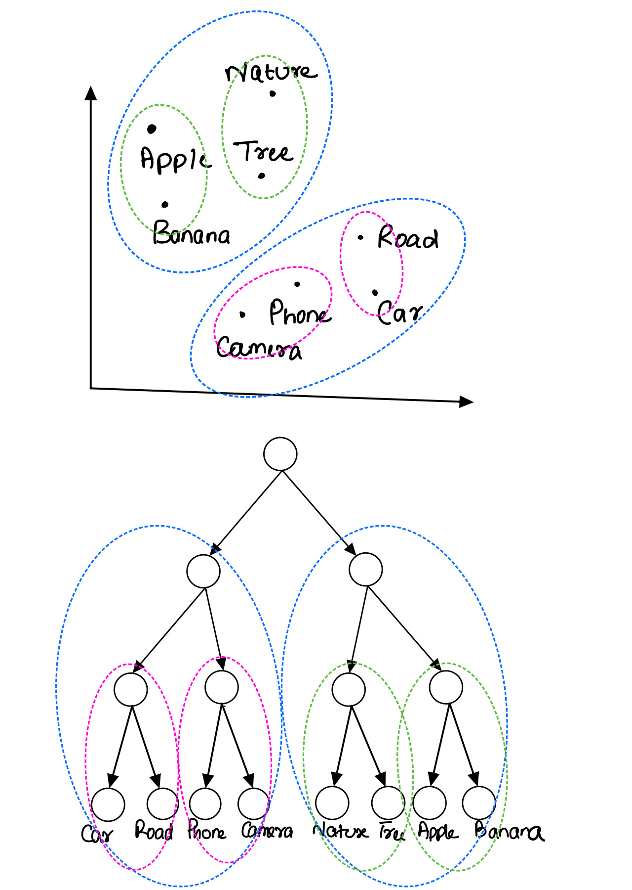
The idea of optimal word assignment in hierarchical softmax is similar. Similar words must be on the same side of a node. For example, apple and banana are better on the same side of a node. Tree A makes more sense than Tree B in the figure below.
Secondly, why is it necessary for the tree to be balanced? The authors say it results in faster training and testing, probably because all the words are at the same level. However, there are implementations of hierarchical softmax using Huffman coding that result in shorter paths for more frequent words.
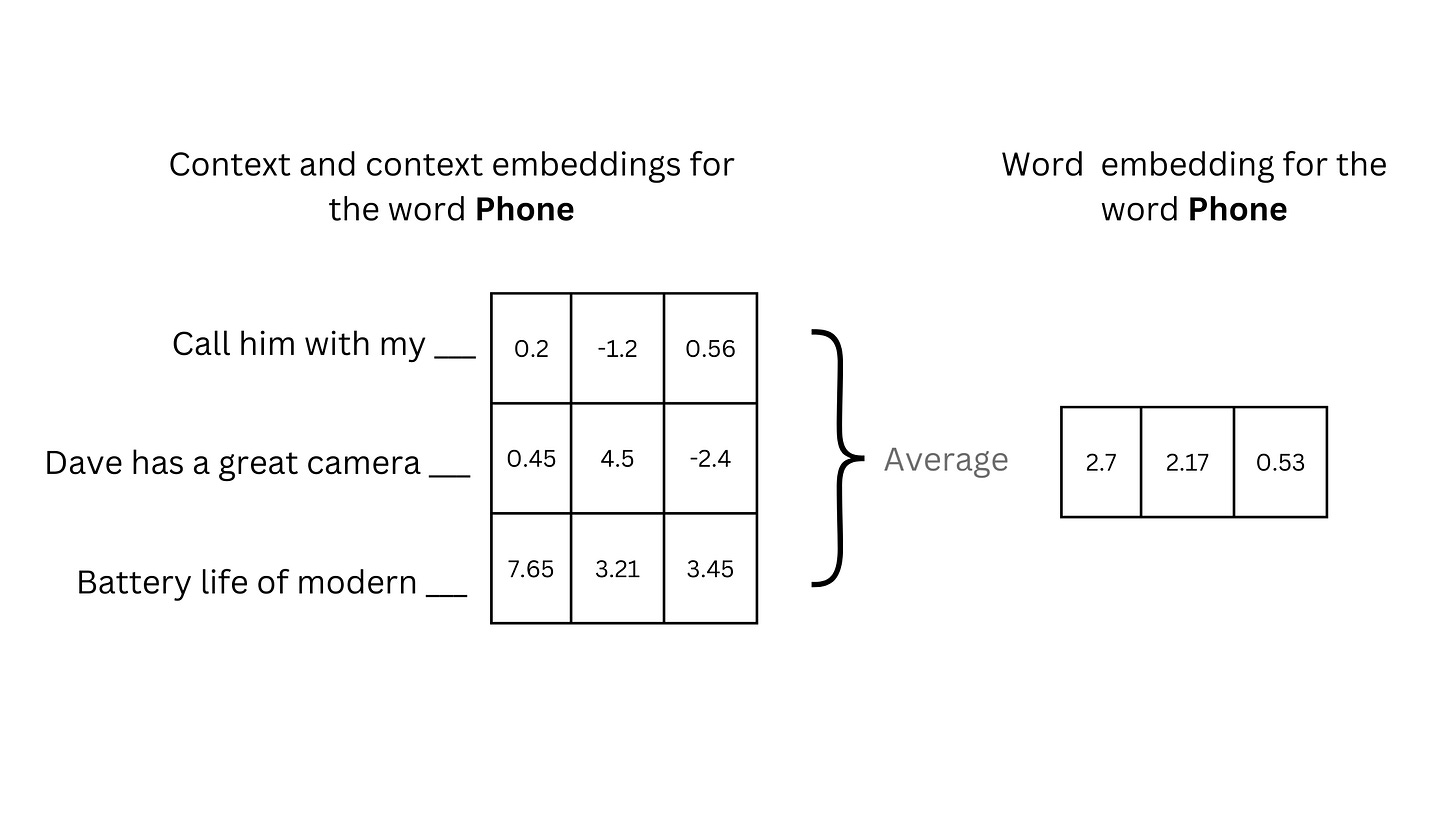
Let's consider the implementation if the idea behind creating the tree is clear. First, create a randomly assigned tree and train the model. At this point, we have trained the word and node embeddings along with the combination weights. Next, we take the training data and collect all contexts for each word in the vocabulary. These contexts are used to generate respective context embeddings. Now, the embedding for the word is treated as the average of these context embeddings instead of the original word embedding.

Once we have word embeddings for each word in the vocabulary, we run the expectation maximization (EM) algorithm to learn two distributions. Each word has a probability of belonging to a distribution. For a cluster, we sort these probabilities computed for each word and create two clusters out of the top 50% and bottom 50%. These sets are assigned on either side of the root node. The process repeats for each child node until we have groups of two words.

This approach directly supports the model training. At any node, split is a function of the context and node embedding. Because the clustering (and hence the assignment) is based on context embeddings, learning the node embedding to separate the two groups is now easier. For any two clusters, the node embedding is approximately the hyperplane that separates the two. In a way, good word assignment leads to faster learning.
Now that the vocabulary is assigned to the tree, the model is trained again.


