Simplest explanation on dynamic programming in RL
Establishing the core vocabulary and concepts in RL, and understanding why dynamic programming is so fundamental to RL.


A refresher in RL
Reinforcement Learning (RL) involves learning how to achieve a certain goal over time in an environment. For example, if the environment is a chess board and an opponent, an agent (computer/algorithm) learns how to win at chess. The way it learns is by interacting with the environment. In this case, it means playing many games against the opponent and trying to win as many times as possible. Upon the completion of an objective, the agent receives a reward. The goal of an agent is to maximize reward in the environment. Depending on the environment and objective, rewards may be received only upon completion of the overall goal or potentially for intermediate steps.
In this article, I focus on a key concept in RL - the application of dynamic programming.
RL’s Basic Vocabulary
Environment - This is where an agent performs actions. The environment consists of rules and constraints that describe what an agent can and cannot do (rules of a game). Whenever an agent takes an action, the environment conveys its result to the agent.
Agent - An entity that interacts with the environment to learn to accomplish a task. It does so by taking actions and figuring out which actions bring it closer to its goal.
State - State is the information the agent can obtain by observing the environment and its own position at any time. In RL, the agent uses the state to decide the best possible action. For example, any placement of chess pieces on the board can qualify as a state.
Reward - Quantifies the quality of action(s) the agent takes. Rewards are aligned with the task that the agent should learn. For example, winning a game yields positive rewards, and losing is negative. Sometimes, the reward is received only if the goal is accomplished; sometimes, the reward is received by taking single actions.
Policy (π(S)) - Dictates the action in a given state. The agent fulfills its goal of maximizing the reward by learning the optimal policy, such as what piece to move, given the current state of the chessboard. This may be an ML model that takes the state as an input and gives probabilities over the action space as an output.
Value function (Vπ(S)) - For any given state S and policy π, what is the expected reward if the agent starts at this state and acts according to π? Measures the potential reward that can be collected from this state.
The agent starts with a certain state, S. Depending on its current state, it takes the best action, a. The environment responds with a new state, S’, and a reward, R. Now, the agent's current state is S’.
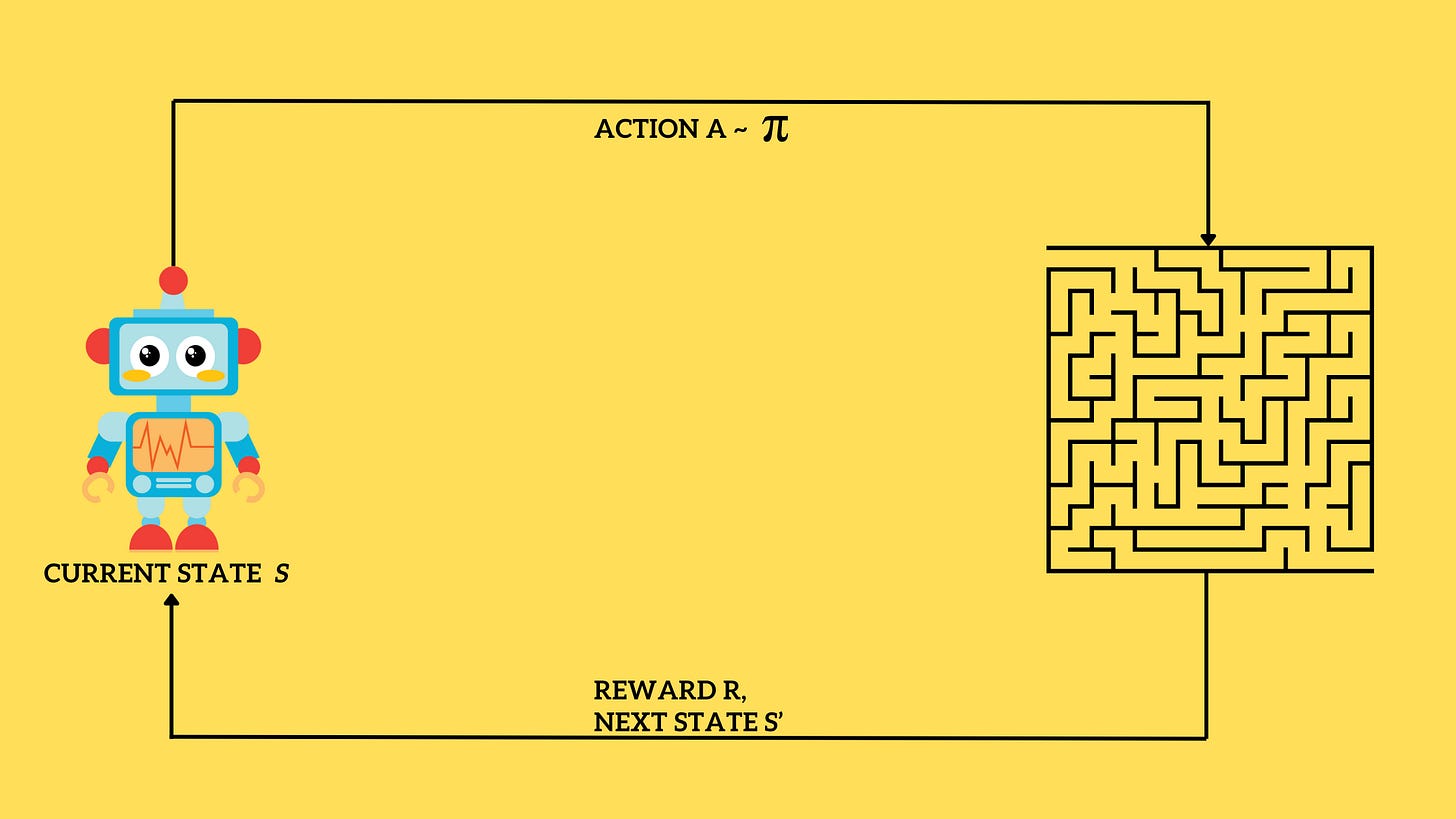
Fig 1. Illustration of an RL agent, and environment and the dynamics. An agent in a state S performs an action (say a move to get out of the maze). As it finishes a step, it is in a new position called S’. Depending on how close the move got to the finish line, it receives a reward R. Now S’ is the current state, and the agent performs an action again. States that lead to a dead end will have a lower value than states that can access a route to the finish line. γ (discount factor) - γ is the discount factor that lies between 0 and 1. It discounts future rewards compared to immediate rewards. In simple terms, future rewards are relatively less important than the immediate reward. For example, the value received by taking N steps with rewards r1, r2, …, rN is
\(V = r_1 + \gamma r_2 + \gamma^2 r_3 + \cdots + \gamma^{N-1} r_N \)If γ is small, the agent tends to take more near-sighted actions. Conversely, larger γ encourages the agent to take far-sighted actions. γ is usually between 0 and 1 because imposing too much far-sightedness makes it harder for the agent to converge to an optimal policy, as it tends to explore excessively. In a way, the agent thinks too much about the future and ignores the reward it gets right now.
Markov Decision Process (MDP) - A common assumption in RL is that the environment dynamics follow a Markov Decision Process (MDP). This means that the current state has enough information for an agent to take the next action. Given the current state, the information from the previous states is irrelevant. This assumption simplifies the agent's learning mechanism.

An important dichotomy in RL: model-free and model-based methods
An important piece of information in any RL problem is whether or not the environment’s model is explicitly known. If so, methods that leverage the environment's structure and dynamics are preferable. Such methods are called model-based methods. The word ‘model’ refers to the environment's model, not an ML model that learns the policy. Generally, such environments have a practically finite number of states.
On the contrary, there are cases where the environment cannot be modeled due to complexity and unpredictability; hence, we can’t exploit its structure. In such cases, we use model-free methods that don’t need the environment’s structure. Most video games like Super Mario are treated as model-free environments. Why? because the number of states — the combination of Mario’s position, the positions of the mushrooms, turtles, etc. —is humongous.
Model-based learning is about planning.
Visibility into the environment is at the heart of model-based learning. A learned agent takes action intending to move to a specific state. This specific state is part of the trajectory it has discovered leads to the highest rewards. To follow this trajectory, it learns to take appropriate actions. In short, the agent plans its success.
On the contrary, model-free methods are used in environments where it is impossible to explore trajectories because of the sheer number of possible states. For example, a self-driving car cannot plan for every possible situation of the road, traffic, and pedestrians. Hence, such methods learn from experience and generalize it. They implicitly learn the approximate model of the environment.
Dynamic programming accelerates planning.
The core idea behind dynamic programming is to reuse intermediate results. For example, consider a mouse navigating a maze. The mouse tries navigating the maze several times. Sometimes, it succeeds; sometimes, it reaches a dead end. As it navigates the maze, it finds itself coming across many intersections. Consider one such intersection that always leads to a dead end. The mouse knows that the moment it reaches this intersection, any further action will lead to a dead end. Although it may take a new path in hopes of reaching the goal, if it encounters this intersection, it must stop right there. It does not need to go down the same road again because the result of doing so is known. Hence, dynamic programming helps avoid redundant computations.
However, how does dynamic programming help us find the most rewarding path? The answer lies in Bellman’s principle of optimality, which says —
Large multi-step control policy must also be locally optimal in every sub-sequence of steps.
To understand the above statement, consider the following equation.
The optimal value at state S is the largest [r + γV(S’)] among all possible next states. Note that r depends on S and S’. In a way, we are working our way backward. Having the optimal value for the next states (all S’s) enables us to compute the optimal value for S. The above equation conveys the idea of dynamic programming used to compute optimal values for a state.
However, it is incomplete and misleading.
First, it ignores the policy and maximizes directly over the state space. In RL, the agent takes action to reach the next state. The next stage results from the action, current state, and the environment. In most cases, we do not have direct access to the next state (1).
Secondly, even if we introduce the action like —
It assumes that taking an action in a state S always leads to a specific S’; otherwise, the above equation doesn’t make sense. It assumes a deterministic mapping exists from (current state, action) → (next state). However, this is not always true. The next state can be probabilistic, i.e., the same (current state, action) pair can lead to different states (for example, a man walking on a slippery surface). Hence, if we claim that the value at a state is high, it must account for all possibilities resulting from an action and not just one of the high-value next state. In parallel, we take actions that have the highest expected reward. Mathematically, we introduce this generalization using p(S’, r | S, a), which indicates the probability of landing in the next state given the (current state, action) pair. The updated equation is —
For action a, we consider all possible next states S’ and the corresponding reward received in the transition. Next, we compute the total reward [r + γV(S’)] and weigh it by the probability of the transition p(S’, r | S, a) for each state S’. Summing this product for all possible states S’ gives us the value of S by taking action a. Lastly, we take action a that maximizes this sum. As an example, consider the following table.
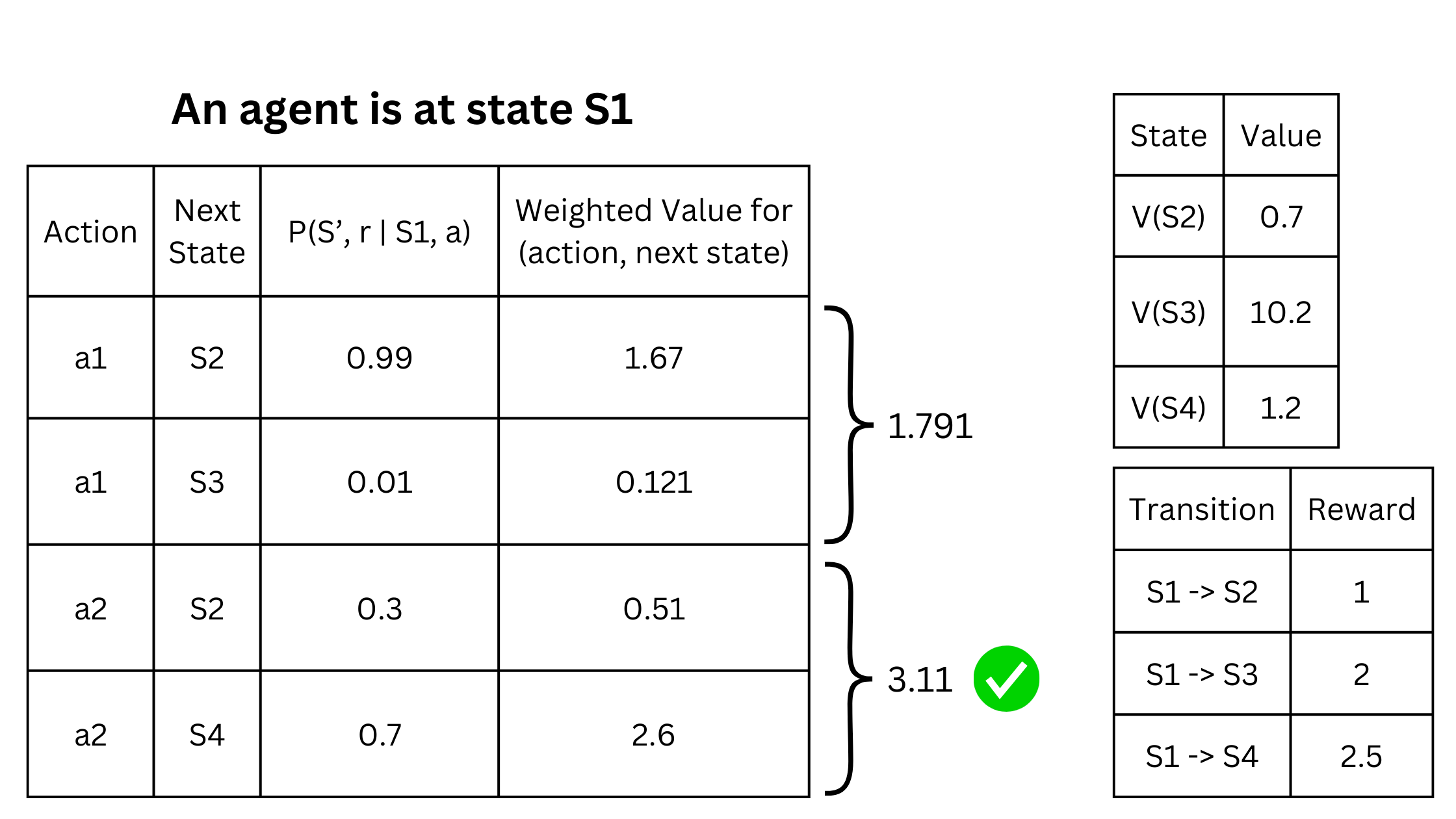
The table to the left describes the possibilities of taking actions a1 and a2 from the current state S1. If the agent takes action a2, it lands in S2 with a probability of 0.3 and S4 with a probability of 0.7. The expected value of S1 if action a2 is taken is
which is
Similarly, the expected value computed from taking the action a1 is 1.791. Comparing these two actions based on their expected value, taking a2 is a wiser choice. Notice that even though taking a1 can lead to S3 with the highest value of 10.2, the expected value of a1 is lesser.
Conclusion
We can explore specific methods now that we have set RL's key nuts and bolts. The next article will explore model-based methods like value and policy iteration.