[Paper Summary] How Google Play Store improved its recommendations using a novel negative sampling technique
Learnings from the paper - Mixed Negative Sampling for Learning Two-tower Neural Networks in Recommendations
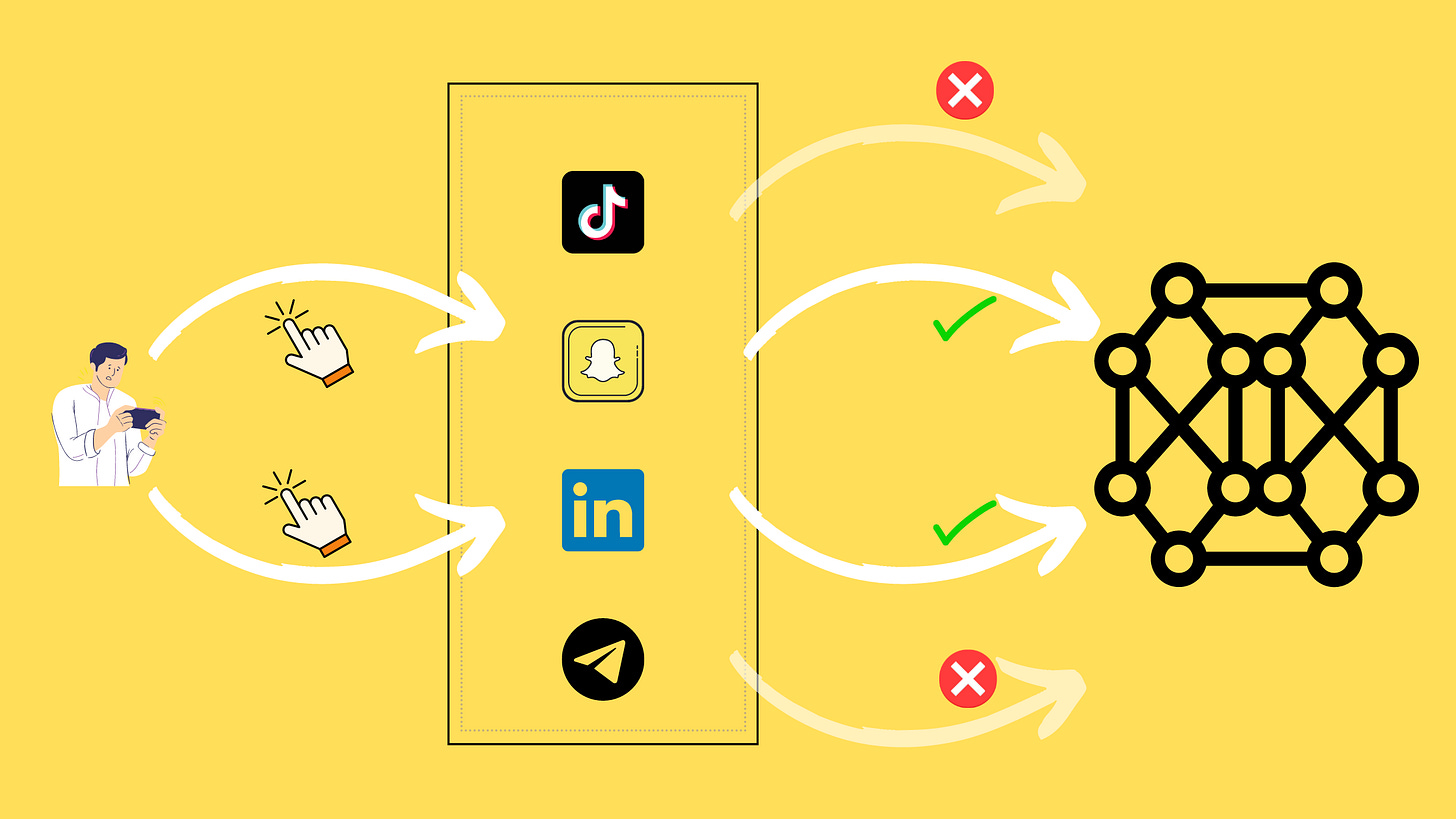
Recommender systems suffer a major deficiency in their feedback loops. When a user interacts with only a few out of many apps on the Play Store homepage, we can only assume their interest in those specific apps. Unfortunately, we lack data on the remaining apps the user did not interact with, even those that weren't displayed altogether. We only have data on the positive class and no explicit records of the negative class when viewed from a binary classification standpoint.
Paper link.
In addition, classical algorithms like matrix factorization do not directly support cold-start settings. One cannot make predictions for a new user using an existing model. At least one click event is required for the user to be included in the model training. Predictions can be produced only when the model is re-trained with the new user’s clicks.
The above two problems can be solved by producing negative examples using negative sampling. The examples produced are not actual feedback from the user but are assumed to be true (explained ahead). Consider a click dataset on the left with userIds and appIds. The training dataset has only three users and three apps. Each row describes which app did a particular user click on. This characterizes our positive class dataset.

We use the rest of the apps to generate negative class examples for a userId in the nth row. In the right table, we have data points from both classes; hence, we can use them for binary classification.
The assumption is that any user is interested in only a small percentage of apps from the universe of apps. Hence, picking an app randomly is more likely to be a negative example than a positive one.
Model Architecture
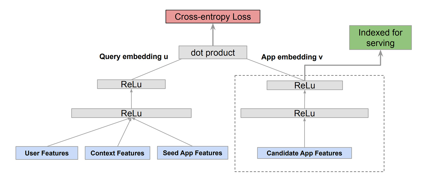
While the negative sampling technique is the paper's main focus, I have included a summary of the model used. The authors use a two-tower DNN as shown in the figure below.
The tower on the left generates query (user) embeddings through a sequence of linear layers with ReLU activation, utilizing a range of user, context, and seed app features as inputs. While the exact meaning of "seed app features" may not be clear, they may refer to previous app installations within a defined period. On the other hand, the right tower also receives app features as inputs through a corresponding sequence of linear layers. The resulting query and app embedding are then utilized to determine the cross-entropy loss.
The right tower is used during inference to get the app embedding for each app, which is then indexed in a vector search DB like faiss, ScaNN, etc. To get the results for a user, the left tower is fed with user, context and seed app features to get the user embedding, which is used to score each app in the vector index.
Negative sampling implementation - Naive version
Large-scale recommender systems have two main stages - Retrieval and Ranking. In the retrieval stage, a model selects a few thousand candidates (in this case appIds) from a corpus of millions. This model aims to ensure the most relevant ones are present in these thousands without bothering about their rank. The ranking stage takes these thousand candidates and re-ranks them so that the most relevant ones are ranked higher. Focusing on the retrieval stage, the problem is formulated as a multiclass classification problem.
For a total appId corpus C, we treat each appId as a separate class. For a click event by a user on an app with a particular appId, the appId ‘class’ will be one, and the rest C-1 classes will have a label 0. The predicted probability for loss calculation is computed as shown in the above figure. However, probability computation involves calculating softmax-like terms over the entire corpus, which is expensive.
To avoid the expensive computations in the above equation, we sample a smaller corpus C’ from the training batch instead of taking the entire corpus C. This sample C’ is sampled based on the occurrence probability of an app in the dataset, represented by Qj. The higher the frequency of an app, the greater the chances of it being selected as a negative sample.
C = [appId_1, appId_2, ...]
N = training data size
count_i = occurence of app_i (C[i])
Q = [count_1/N, count_2/N, ... count_C/N]
batch = [(userId_1, appId_1), (userId_2, appId_2), ...]
K = size of sample corpus C'

for userId, appId in batch:
    neg_sample_appIds = random.sample(C, weights=Q, n_samples=K)
    if appId in neg_sample_appIds:
        neg_sample_appIds.remove(appId) #remove positive appId from neg samples

    app_tower_inputs = [appId] + neg_sample_appIds
    labels = [1] + len(neg_sample_appIds)*[0]
    user_embedding = model.get_user_embedding([userId])
    app_embedding = model.get_app_embedding(app_tower_inputs)
    scores = cosine(user_embedding, app_embedding)
    loss = loss_fn(labels, score)
The problem with this approach is that we need to sample C’ for every positive pair and make a forward pass through the right tower, which is still costly.
Such a negative sampling is biased.
Another problem is that such a sampling strategy suffers from selection bias. The training data is biased towards popular apps. Less popular or long-tailed apps have fewer instances of clicks and hence don’t appear nearly as frequently and have a smaller Qj. Since popular appIds are over-represented in positive pairs, they are over-represented in the negative pairs too. Conversely, the long-tailed apps are under-represented in positive and hence negative pairs. As a result, the model does not learn enough about the long-tailed apps due to a lack of training examples.

As mentioned earlier, we treat the problem like a multi-class classification problem. The softmax calculation is tainted with information from the training distribution (manifested as popular apps appearing more often in the softmax calculation).
A common resolution to this problem is to add a correction term. In this case, it is the following transformation.
Here, Q is the item-frequency probability in the training data. Intuitively, the exponential term is weighed by an inverse of its probability (separate and simplify the log exponential correction). If the item is less frequently occurring, the inverse weight is larger, correcting the bias caused by underrepresentation.
However, this correction is applied after sampling, meaning long-tailed apps are still under-represented. The correction only ensures that popular apps don’t get too much importance. The authors argue they have a better way to eliminate the selection bias using Mixed Negative Sampling (covered ahead).
In-batch negative sampling
Instead of especially sampling C’, which is expensive, we can use the training batch to create negative samples. For each positive pair in the batch, appIds from other pairs in the same batch can be used as negative samples. It is not necessary to sample C' separately. Additionally, there is no need to perform specific forward passes for negative samples since it is already included when appIds are part of positive pairs in a batch.
Although this solves the expensive computation problem, the under-representation of long-tail apps remains problematic.
Mixed Negative Sampling (MNS)
The idea proposed in the paper involves two sources of negative samples: unigram sampling (in-batch sampling) and uniform sampling. In the latter, instead of sampling from batches where long-tail apps are under-represented, we sample from the index of appIds. Since the index is a set of appIds, each app has an equal chance of getting sampled. The long-tailed apps will have a greater chance of being included in the training data as negatives than in-batch sampling.
B and B’ are batch sizes for in-batch and index-based negative samples. Total batch size being B + B’. The blue section on the label matrix represents the labels obtained through in-batch sampling, while the orange section corresponds to index-based sampling.
Evaluation
The authors trained a model on 30 days of Google Play’s logs and evaluated it on the 31st day. This exercise was performed seven times, each time moving the training and the evaluation window by one day.
Improved recall@K - The authors report results of the three models
MLP with Sampled Softmax - Two-layer DNN with hidden layer sizes [1024, 128]
Two-tower with Batch Negatives - Two-tower with [512, 128] hidden-sized tower, trained with in-batch negative sampling
Two-tower with MNS - Two-tower with [512, 128] hidden-sized tower, trained with MNS.
Note that each model has roughly the same parameters and effective batch size. In the case of MNS, the batch is 50% index and 50% in-batch sampled.
It is worth noting that in-batch sampling performs worse than MLP with sampled softmax. This could be because sampled softmax selects negative sample appIds from the whole corpus instead of a batch.
Improved retrieval set - The authors observed that the retrieved candidates from the model improved after adding index-based negative samples. Since they do not appear frequently in training samples, low-quality apps are not demoted as frequently as they should be. However, an index-based sampling includes them more frequently as negative samples.
Optimal B and B’ ratio - For a fixed B=1024, the authors compiled results for varying B’. Increasing B’ improves the metrics only to a certain limit. This makes sense as larger B’ will make the training batch too close to a uniform distribution.
Conclusion
The paper points out the selection bias in conventional negative sampling techniques and how to mitigate it. Overall, the technique is not too complex to apply on top of in-batch negative sampling. Packages like tensorflow-recommmenders have ready APIs like Retrieval to configure such tasks.
What papers would you like me to cover next? Feel free to drop some suggestions in the comments.


